International House Price Nowcast

Overview

The purpose of this analysis is to provide timely updates of the real house prices in different countries. The publication lag of the International House Price Database (Dallas Fed) used in the International Housing Observatory (IHO) is of around 3 months. This presents an opportunity to forecast the current quarter using higher frequency data (i.e., monthly indicators). As such, the IHO Global Housing Outlook reports, which analyze the latest house price data release, provides a combination of recent trends with an updated assessment of house price developments based on model estimations.

Variables

The model variables are divided into quarterly and monthly series. When needed, variables are seasonally adjusted with X13-ARIMA-SEATS and transformed to be in terms of period-on-period log growth rates. The following table describes the scope of the analysis for the US:

Mnemonic	Variable Description	Sector	Type	Frequency	SA	DIFF
RHPI	Real House Price Index	Housing	Hard	Q	No	Yes
GDP	Real GDP	Activity	Hard	Q	No	Yes
ASP	Average Sales Price for New Houses Sold	Housing	Hard	M	Yes	Yes
PER	Number of Permits for New Privately-owned Single-family Houses	Housing	Hard	M	No	Yes
HOU	Number of New Privately-owned Single-family Houses Started	Housing	Hard	M	No	Yes
HSN	Number of New One-family Houses Sold	Housing	Hard	M	No	Yes

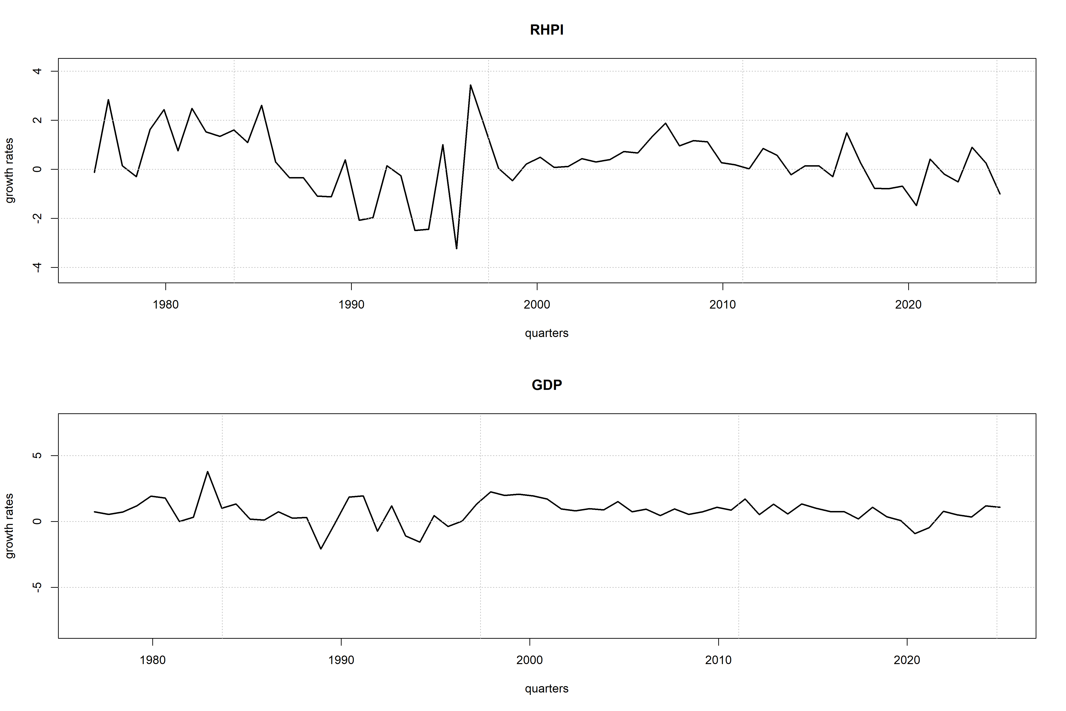
Source: Dallas Fed International House Price Database, FRED, and own calculations.

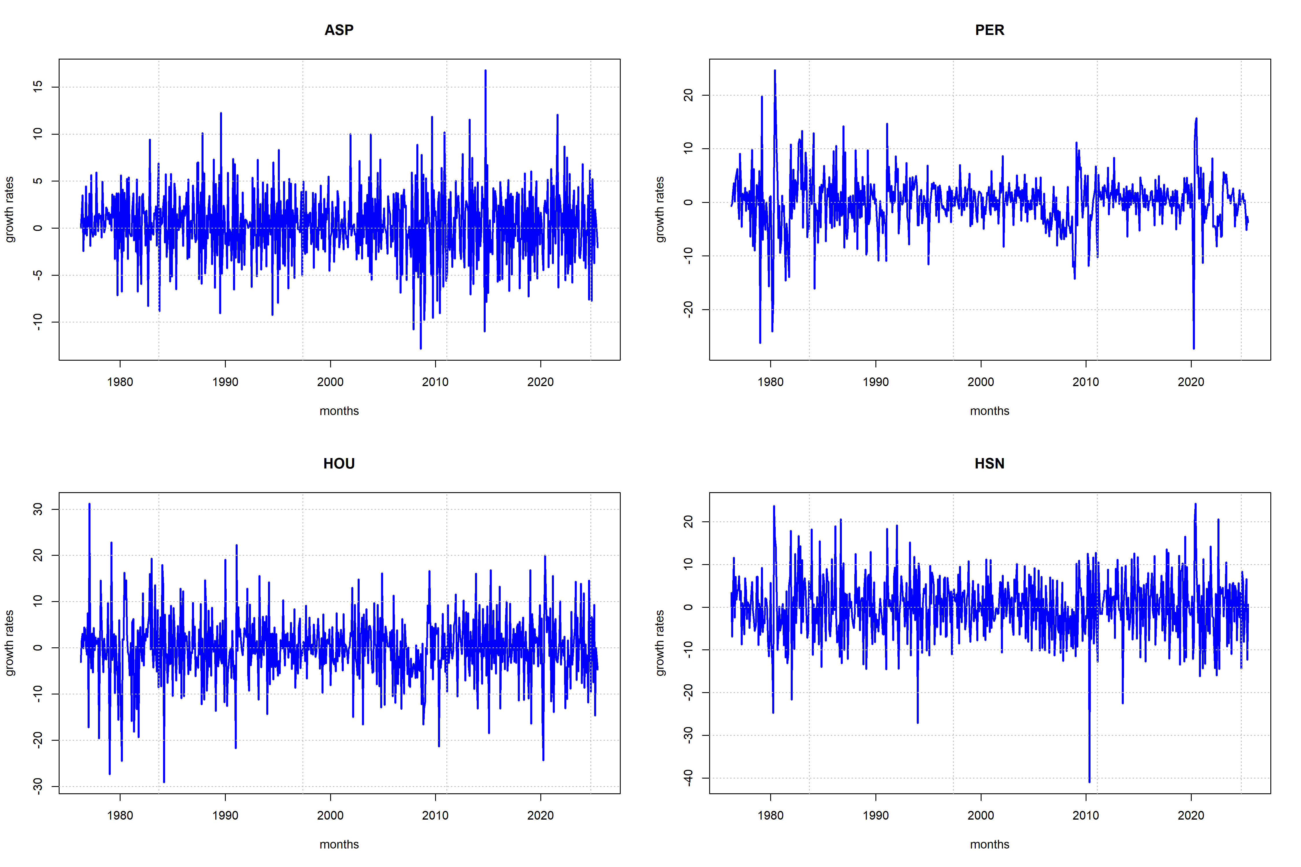
Source: Dallas Fed International House Price Database, FRED, and own calculations.

Model

The main forecasting model is a mixed-frequency dynamic factor model estimated with classical methods (nowcast). The benchmarks to beat are (i) a random walk (RW), (ii) an autoregressive model of order 1 (AR1).

Model Description

For illustration purposes the following equations describe a simplified mixed-frequency dynamic factor model (i.e., 1 quarterly and 2 monthly variables):

Notation:

\( x_{Q,t} \) = target quarterly frequency variable with month-to-quarter growth rate mapping measured in months.
\( x_{M,t} \) = target quarterly frequency variables measured in months.
\( y_{M_j,t} \) = j-th monthly frequency variables measured in months.

DFM equations:

\begin{align*} x_{Q,t} &= \frac{1}{3}x_{M,t} + \frac{2}{3}x_{M,t-1} + x_{M,t-2} + \frac{2}{3}x_{M,t-3} + \frac{1}{3}x_{M,t-4}, \\ x_{M,t} &= \gamma_{M,t} f_t + e_{M,t}, \\ x_{Q,t} &= \frac{1}{3} \gamma_{M} f_{t} + \frac{2}{3} \gamma_{M} f_{t-1} + \gamma_{M} f_{t-2} + \frac{2}{3} \gamma_{M} f_{t-3} + \frac{1}{3} \gamma_{M} f_{t-4} \\ &+ \frac{1}{3} e_{M,t} + \frac{2}{3} e_{M,t-1} + e_{M,t-2} + \frac{2}{3} e_{M,t-3} + \frac{1}{3} e_{M,t-4}, \\ y_{M_1,t} &= \gamma_{M_1,t} f_t + e_{M_1,t}, \\ y_{M_2,t} &= \gamma_{M_2,t} f_t + e_{M_2,t}, \\ f_{t} &= \phi_1 f_{t-1} + \phi_2 f_{t-2} + \varepsilon_{f,t}, \quad \varepsilon_{f,t} \sim N(0, 1), \\ e_{j,t} &= \psi_{j,1} e_{j,t-1} + \psi_{j,2} e_{j,t-2} + \eta_{j,t}, \quad \eta_{j,t} \sim N(0, \sigma^2_{\eta_j}), \quad j = M, M_1, M_2. \end{align*}

State-space representation:

Measurement equation \(\rightarrow\) \( y_t = H' h_t \):

\[ \begin{bmatrix} x_{Q,t} \\ y_{M_1,t} \\ y_{M_2,t} \end{bmatrix} = \begin{bmatrix} \frac{1}{3} \gamma_M & \frac{2}{3} \gamma_M & \gamma_M & \frac{2}{3} \gamma_M & \frac{1}{3} \gamma_M & \frac{1}{3} & \frac{2}{3} & 1 & \frac{2}{3} & \frac{1}{3} & 0 & 0 & 0 & 0 \\ \gamma_{M_1} & 0 & 0 & 0 & 0 & 0 & 0 & 0 & 0 & 0 & 1 & 0 & 0 & 0\\ \gamma_{M_2} & 0 & 0 & 0 & 0 & 0 & 0 & 0 & 0 & 0 & 0 & 0 & 1 & 0 \end{bmatrix} \begin{bmatrix} f_{t} \\ f_{t-1} \\ f_{t-2} \\ f_{t-3} \\ f_{t-4} \\ e_{M,t} \\ e_{M,t-1} \\ e_{M,t-2} \\ e_{M,t-3} \\ e_{M,t-4} \\ e_{M_1,t} \\ e_{M_1,t-1} \\ e_{M_2,t} \\ e_{M_2,t-1} \end{bmatrix} \]

Transition equation \(\rightarrow\) \( h_t = F h_{t-1} + v_t \):

\[ \begin{bmatrix} f_{t} \\ f_{t-1} \\ f_{t-2} \\ f_{t-3} \\ f_{t-4} \\ e_{M,t} \\ e_{M,t-1} \\ e_{M,t-2} \\ e_{M,t-3} \\ e_{M,t-4} \\ e_{M_1,t} \\ e_{M_1,t-1} \\ e_{M_2,t} \\ e_{M_2,t-1} \end{bmatrix} = \begin{bmatrix} \phi_1 & \phi_2 & 0 & 0 & 0 & 0 & 0 & 0 & 0 & 0 & 0 & 0 & 0 & 0\\ 1 & 0 & 0 & 0 & 0 & 0 & 0 & 0 & 0 & 0 & 0 & 0 & 0 & 0\\ 0 & 1 & 0 & 0 & 0 & 0 & 0 & 0 & 0 & 0 & 0 & 0 & 0 & 0\\ 0 & 0 & 1 & 0 & 0 & 0 & 0 & 0 & 0 & 0 & 0 & 0 & 0 & 0\\ 0 & 0 & 0 & 1 & 0 & 0 & 0 & 0 & 0 & 0 & 0 & 0 & 0 & 0\\ 0 & 0 & 0 & 0 & 0 & \psi_{M,1} & \psi_{M,2} & 0 & 0 & 0 & 0 & 0 & 0 & 0\\ 0 & 0 & 0 & 0 & 0 & 1 & 0 & 0 & 0 & 0 & 0 & 0 & 0 & 0\\ 0 & 0 & 0 & 0 & 0 & 0 & 1 & 0 & 0 & 0 & 0 & 0 & 0 & 0\\ 0 & 0 & 0 & 0 & 0 & 0 & 0 & 1 & 0 & 0 & 0 & 0 & 0 & 0\\ 0 & 0 & 0 & 0 & 0 & 0 & 0 & 0 & 1 & 0 & 0 & 0 & 0 & 0\\ 0 & 0 & 0 & 0 & 0 & 0 & 0 & 0 & 0 & 0 & \psi_{M_1,1} & \psi_{M_1,2} & 0 & 0\\ 0 & 0 & 0 & 0 & 0 & 0 & 0 & 0 & 0 & 0 & 1 & 0 & 0 & 0\\ 0 & 0 & 0 & 0 & 0 & 0 & 0 & 0 & 0 & 0 & 0 & 0 & \psi_{M_2,1} & \psi_{M_2,2}\\ 0 & 0 & 0 & 0 & 0 & 0 & 0 & 0 & 0 & 0 & 0 & 0 & 1 & 0 \end{bmatrix} \begin{bmatrix} f_{t-1} \\ f_{t-2} \\ f_{t-3} \\ f_{t-4} \\ f_{t-5} \\ e_{M,t-1} \\ e_{M,t-2} \\ e_{M,t-3} \\ e_{M,t-4} \\ e_{M,t-5} \\ e_{M_1,t-1} \\ e_{M_1,t-2} \\ e_{M_2,t-1} \\ e_{M_2,t-2} \end{bmatrix} + \begin{bmatrix} \varepsilon_{f,t} \\ 0 \\ 0 \\ 0 \\ 0 \\ \eta_{M,t} \\ 0 \\ 0 \\ 0 \\ 0 \\ \eta_{M_1,t} \\ 0 \\ \eta_{M_2,t} \\ 0 \end{bmatrix} \]

Forecast

Dynamic Factor Model
Autoregressive Model

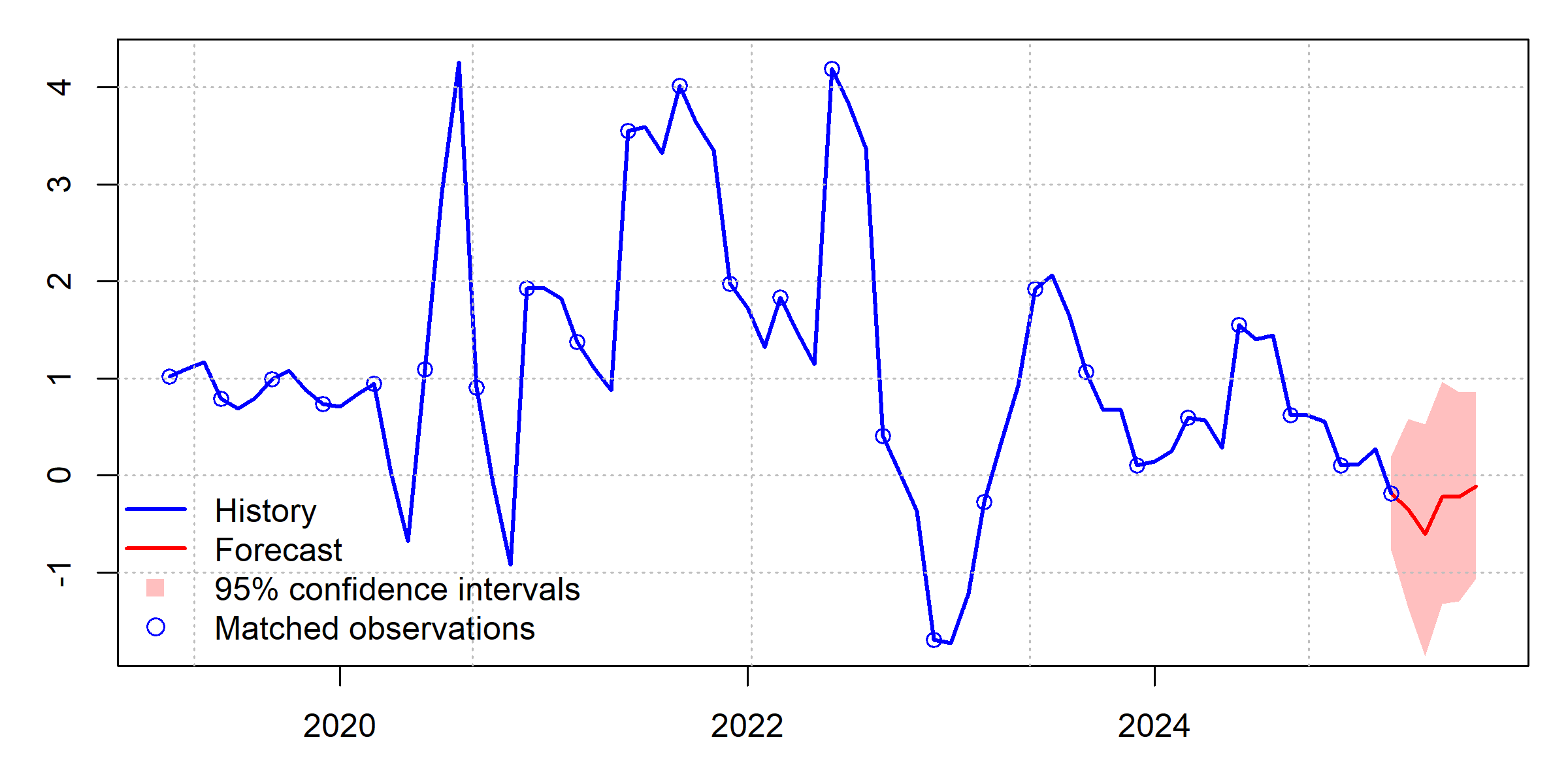
Note: Confidence intervals are computed using Wild boostraps with Rademacher multipliers.

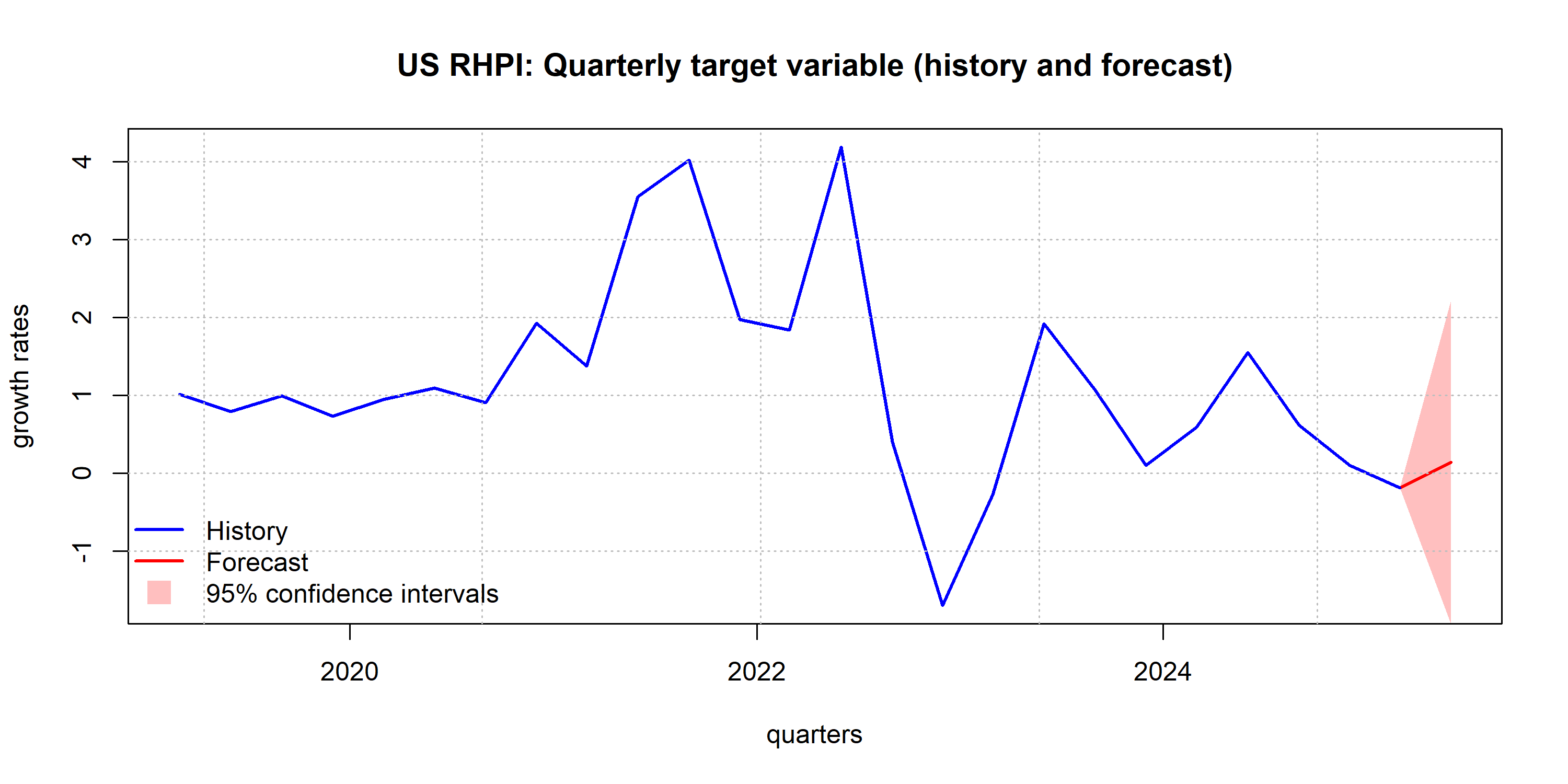
Note: Confidence intervals are computed in a standard way.

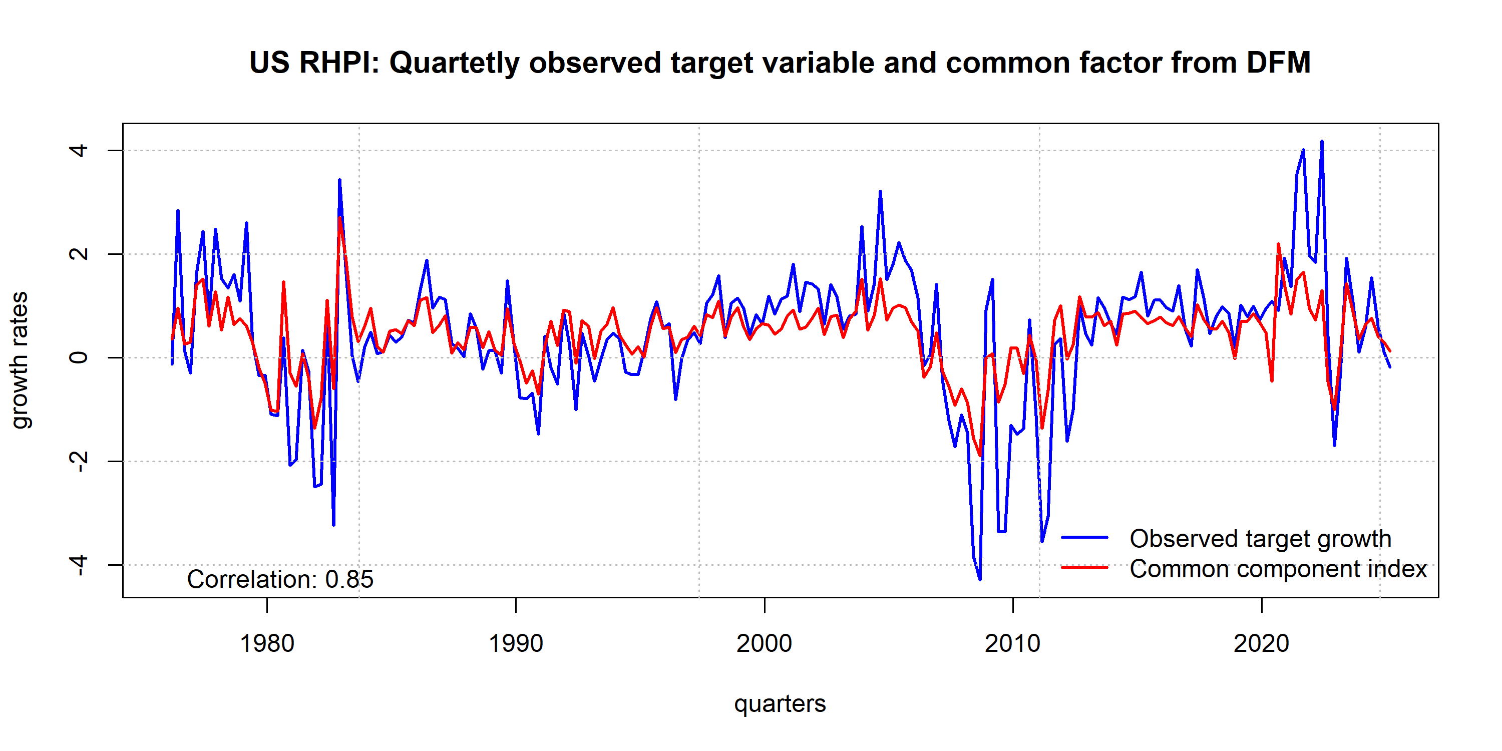
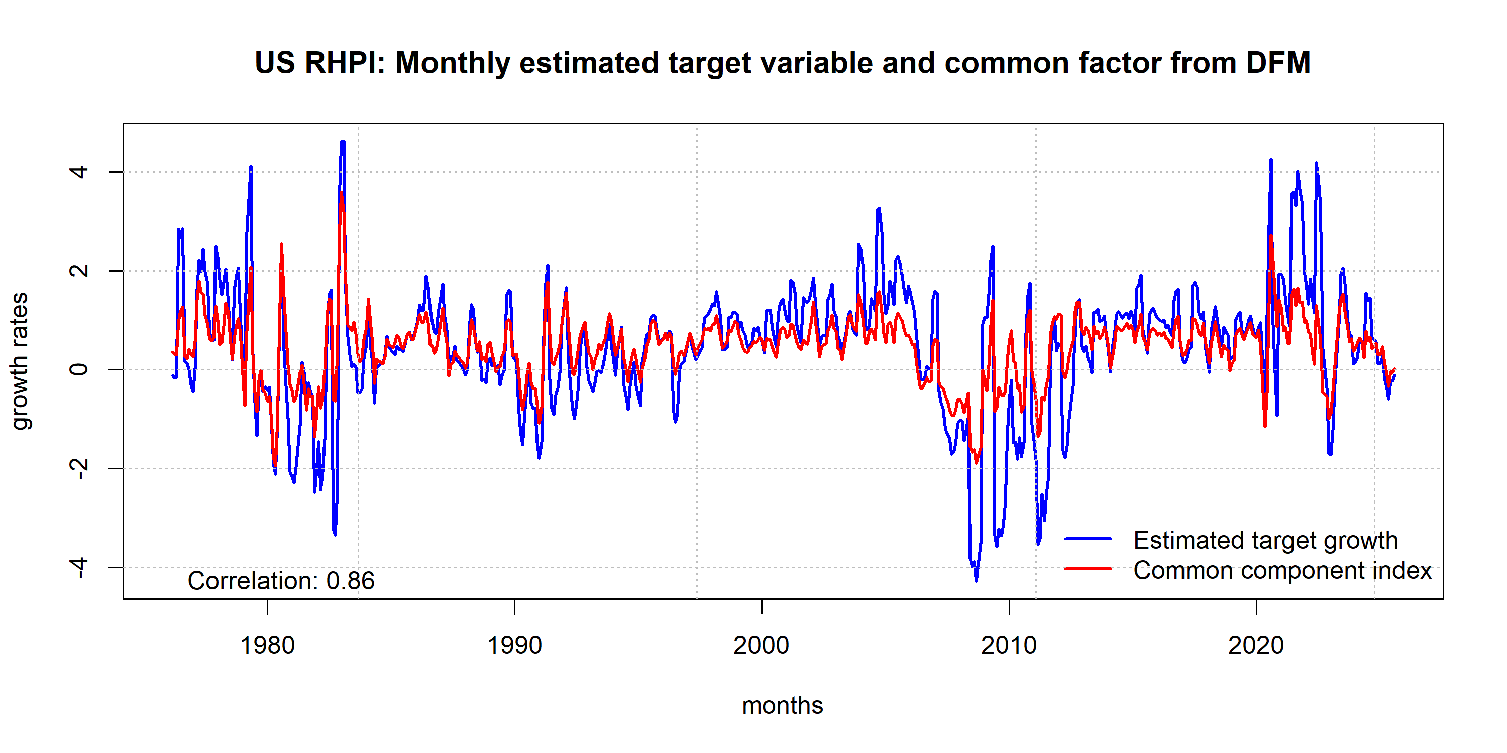
Validation

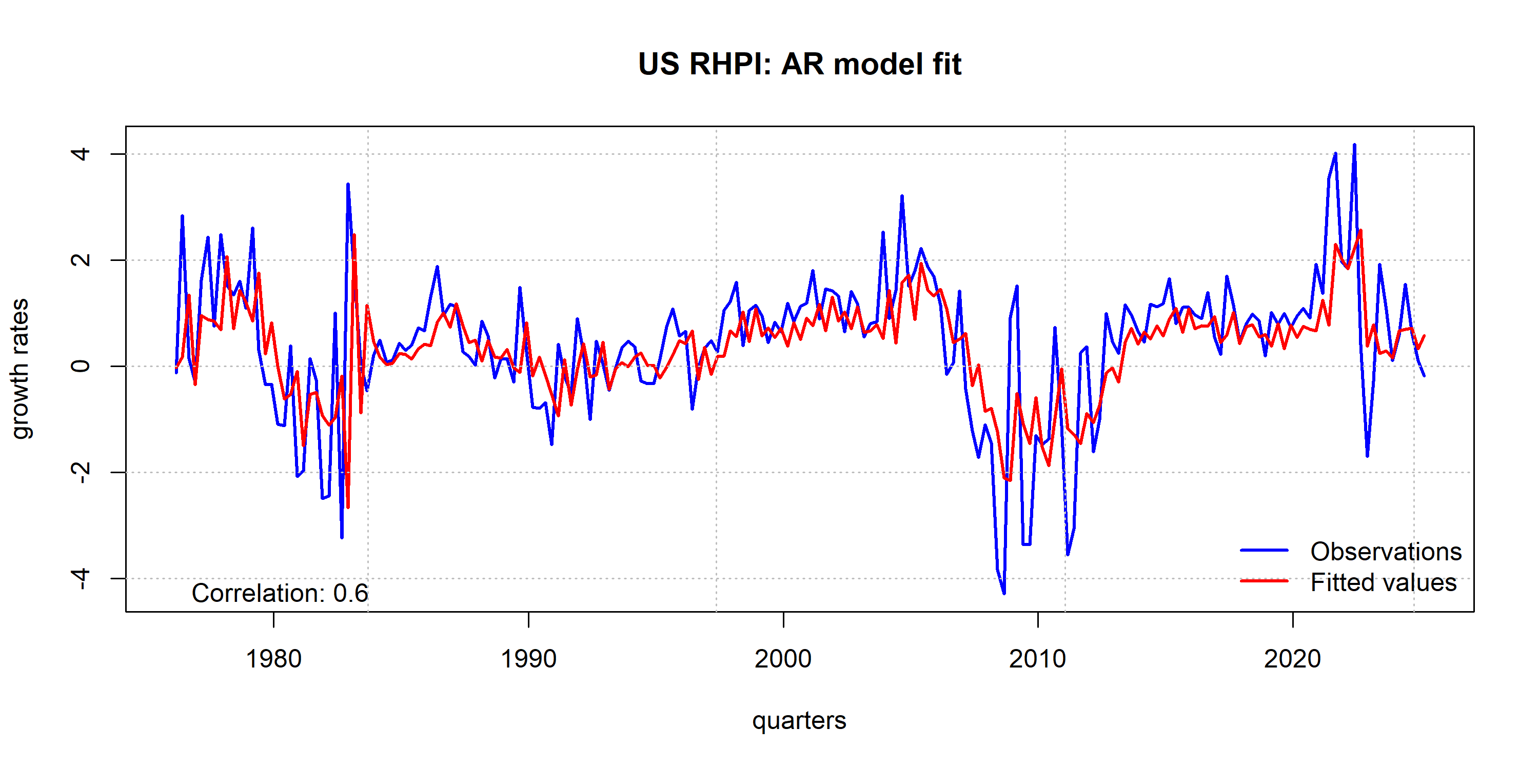
The model validation comprises two exercises. The first one is the in-sample comparison between the observed target variable and the predicted values from the respective model.

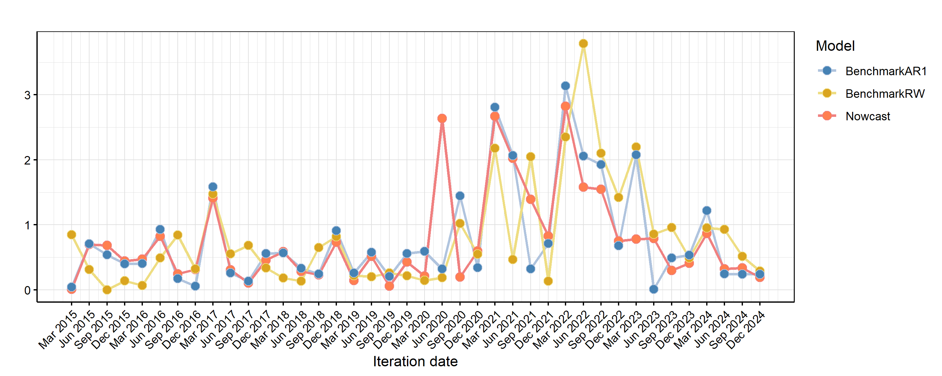
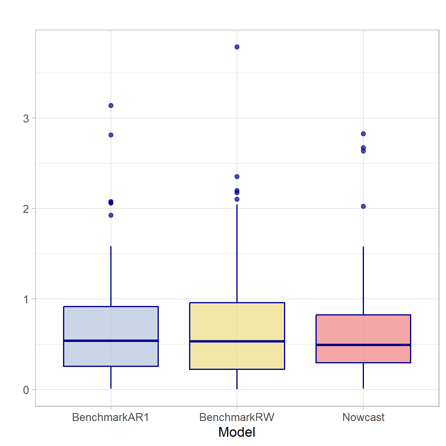
The second exercise is more relevant for forecasting purposes. For the periods 2015Q1-2025Q1 each of the competing models is estimated and then used to forecast the target variable 1-step ahead. The forecast value is compared to the actual observation that period. For example, in the first iteration the model is estimated until 2015Q1 to forecast 2015Q2. Then, the forecast for 2015Q2 is compared to the 2015Q2 observation. This is done iteratively on an expanding window up to the last estimation period of 2024Q4. The forecast accuracy metric is the root mean squared error (RMSE) where lower values indicate a more accurate forecast (i.e., smaller forecast error). This is a pseudo out-of-sample exercise since revised data is used which might be different from the information the forecaster had at the time of doing the forecast.